
Hay
Everyone’s favourite querying language can do more than fetch data to analyse in Python. I firmly believe that in the darkest timeline people use SQL to do everything from developing apps to creating mission critical artificial intelligence.
SQL is easy to pick up and do cool things with, which makes it a good stepping stone for anybody non-technical that wants to make data-driven decisions or fetch data from a table somewhere.
This should be practical and take you on a SQL journey after which you can incorporate it into your own workflow. I’ll try to start simple but move quickly.
SQL stuff you’ll need
My workflow is set up for scientific computing and data sciency things. I recommend the following, but you can always use a terminal.
- Azure Data Studio, it’s a nice tool much like Jupyer Notebooks.
- Note that you can make SQL queries in Jupyer using %magic methods but it’s not a nice user experience.
- Data Studio notebooks are actually iPython notebooks but with an SQL kernel.
- Download : https://docs.microsoft.com/en-us/sql/azure-data-studio/download-azure-data-studio?view=sql-server-ver15
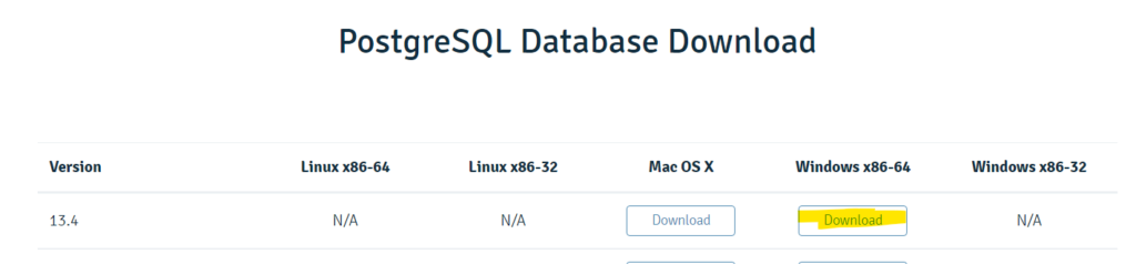
- Some kind of database, I recommend Postgres.
- Download: https://www.postgresql.org/download/
How to SQL? ?
Install Postgres or have the credentials for some other server you want to use. I used the installer for the latest version of Postgres.
I installed all the components.
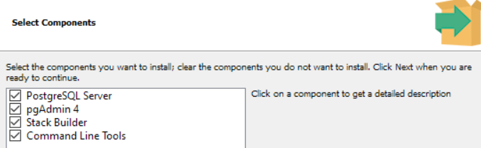
pgAdmin is nice to have but we won’t use it, it is a graphical user interface to manage your database. Makes it easy to import random .CSV files as tables. You can do a lot of that in Azure Data Studio.
You don’t need to install Stack Builder unless you also want to install an older version of Postgres after.
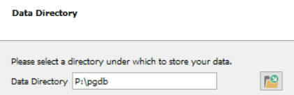
Pick a location to store the data, I wanted it on another drive.
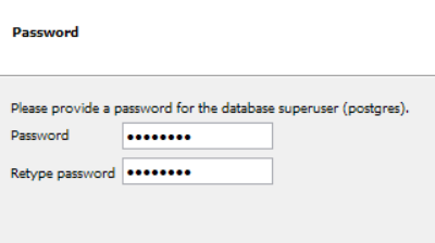
Pick password for password, obviously.
The rest of the user flow is self explanatory, I left the default port and localisation options. I chose not to open Stack Builder upon exit.
Connecting to the database server
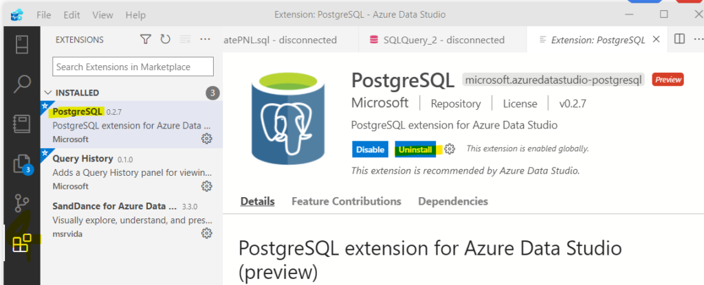
Open Azure Data Studio, and click the blocks on the left panel in the UI to download and install the PostgreSQL extension.
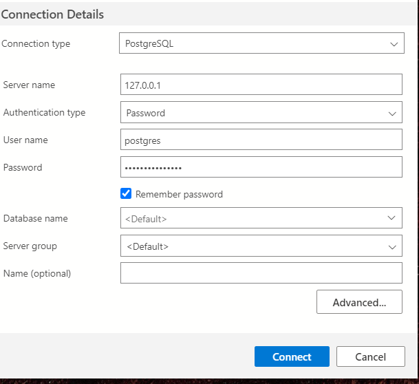
Cool, now we can connect to the database we had installed. Hopefully you remember your password.
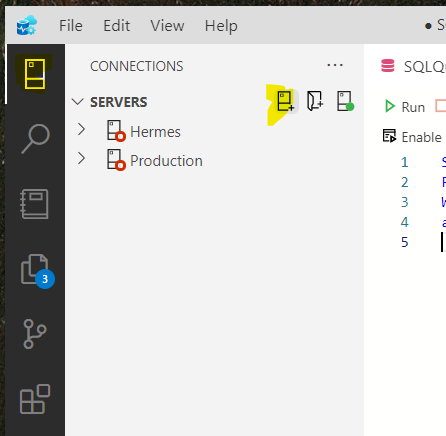
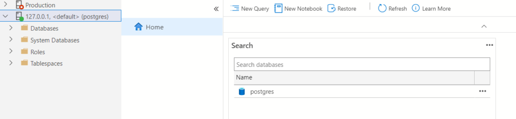
If you see it with a green dot on the left panel then it worked. ??
Notice the New Query and New Notebook options. You can also make a New Notebook by clicking file in the title bar (the top bar).
Creating and querying a table
I clicked new notebook and now I’ll create a table. Google has ridiculous amounts of information on creating tables, the code is also readable and comprehensible.
Run this and see the magic happen.
CREATE TABLE Persons (
    PersonID int,
    LastName varchar(255),
    FirstName varchar(255),
    Address varchar(255),
    City varchar(255)
);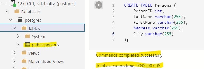
We created a table called Persons with five columns. The pairs inside the create table function represent the column name and their data type. Int is an integer while varchar is a string with a 255 character limit. Feel free to explore other data types.
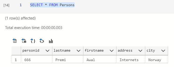
Add an entry to the empty table. It follows this pattern:
INSERT INTO table_name (column1, column2, column3, …)
VALUES (value1, value2, value3, …);
INSERT INTO Persons
VALUES (666, 'Premi', 'Awal', 'Internets', 'Norway');
You can use * to select everything in a table.
SELECT * FROM Persons
If you are somewhat OCD then you can drop that table since we won’t be using it. The data is boring.
DROP TABLE Persons
Importing a useful table
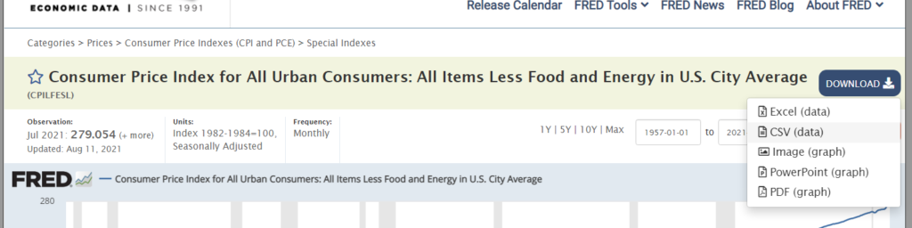
Maybe you already have a dataset you want to analyse. I’m going to download CPI data from the Federal Reserve Bank of St. Louis in .CSV format.
I picked this dataset because it only has two columns, making it easy to understand. We’ll extend the number of columns by joining tables later.
We’ll do something slightly advanced and make it create it’s own primary key using the SERIAL data type thus adding a third column and use the date type.
Put as little thought as possible into the column names like a good data engineer.
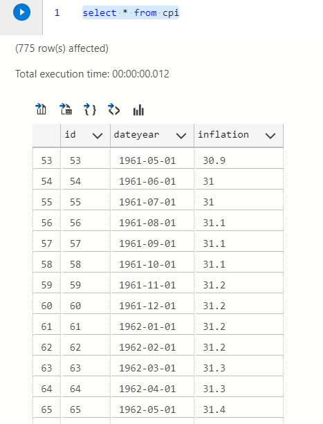
Create Table cpi(
  id SERIAL PRIMARY KEY,
  dateyear date,
  inflation numeric
);
We can import the .CSV using COPY and picking the correct table and columns. Replace the address to the location of your .CSV file.
COPY cpi(dateyear,inflation)
FROM 'P:\Drive\Blogs\SQL for everyone\CPILFESL.csv'
DELIMITER ','
CSV HEADER;
select * from cpi
Now we can actually move on to more interesting stuff.
Intro to intro to joins
Kidding, this isn’t interesting. Maybe no introduction to SQL will be complete without joins since they allow you to do interesting analysis later.

- Left join keeps all the data from the first table but only joins data from the second table that match some column.
- Right join does the same for the other table.
- Inner join returns only the data that match some column in both tables.
- Outer join will join the tables but include unmatched rows from both tables.
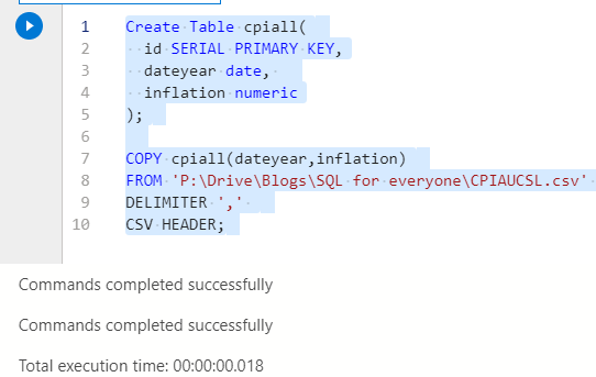
We’ll get another dataset from the FED website. The CPI table from earlier does not include food and energy, we will get the data which includes those.
Import this new dataset just like before.
Create Table cpiall(
  id SERIAL PRIMARY KEY,
  dateyear date,
  inflation numeric
);

COPY cpiall(dateyear,inflation)
FROM 'P:\Drive\Blogs\SQL for everyone\CPIAUCSL.csv'
DELIMITER ','
CSV HEADER;
Don’t be like me and mix upper and lower case SQL syntax. Most places use UPPERCASE FOR SQL and lowercase for properties in the table. It’s less relevant when your editor uses colours but it’s convention.
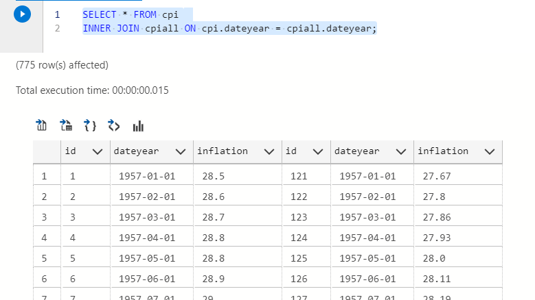
Try out some joins. It’ll have to be on date since it is the only column with shared data.
SELECT * FROM cpi
INNER JOIN cpiall ON cpi.dateyear = cpiall.dateyear;
I used to do my inner joins using WHERE, which is also correct. But was told it isn’t explicitly understood when someone else is reading the code.
This is an inner join using WHERE.
SELECT *
FROM cpi as c, cpiall as a
WHERE c.dateyear = a.dateyear
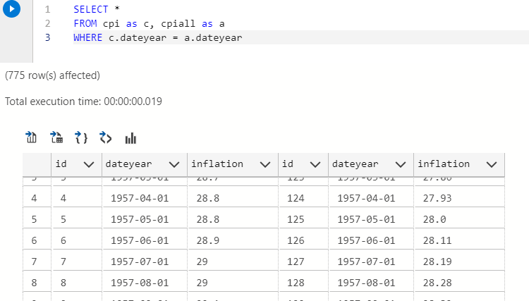
They return the same result but be mindful of others that read your work. Little thought is given to usability with code but it’s appreciated by others.
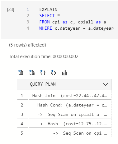
If you aren’t sure whether two queries return the same result use this pro-tip – EXPLAIN shows the execution plan for your query. If two queries have an identical execution plan then they probably return the same stuff.
Examining the CPI dataset in SQL
Nice work, now we move to more advanced querying.
There is a functionality in Postgres called View. Views allow calling a huge query as though it was a table. When a view is called then the query runs and returns the result. It helps maintain neat and reusable code.
There is something called a materialised view too, which is a view but it can be scheduled and the data gets stored on the server. The advantage being it does not have to run the query when called but return the stored data. The disadvantage being the data might not be the latest available. Materialised views also have other restrictions depending on which database you use, we won’t be using them.
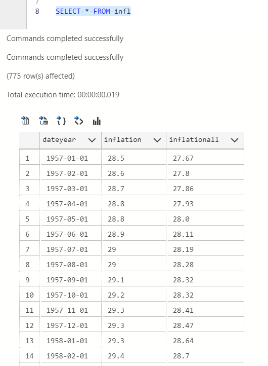
We’ll create a View called ‘infl’ that returns the join without redundant columns.
CREATE VIEW infl AS
SELECT c.dateyear, c.inflation,a.inflation as inflationall
FROM cpi as c, cpiall as a
WHERE c.dateyear = a.dateyear;
You can query the view and be concise. Or better yet, join other tables with a view.
SELECT * FROM infl
Now, as promised the interesting stuff without the deception.
Finding the annual inflation average
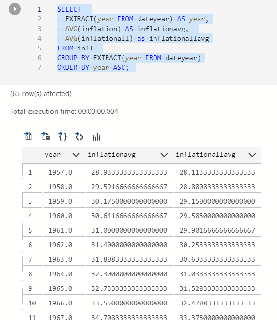
If you want to know what the CPI numbers were per year then we can group by the year and use the average function. It is possible to group this way by extracting the year from the date data type.
CREATE VIEW inflmean AS
SELECT
  EXTRACT(year FROM dateyear) AS year,
  AVG(inflation) AS inflationavg,
  AVG(inflationall) as inflationallavg
FROM infl
GROUP BY EXTRACT(year FROM dateyear)
ORDER BY year ASC;
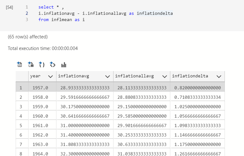
Adding a delta column between inflation numbers
Maybe it’s interesting to see how Food and Energy contribute to the inflation number. We can do arithmetic in queries.
select * ,
i.inflationavg - i.inflationallavg as inflationdelta
from inflmean as i
Calculating moving averages
This is quite common in finance, using a short and long period moving average to see momentum. We’ll use a 3 month and 6 month moving average window. I’ll add the round function to only show 2 decimal places.
You can use OVER to pick a window BETWEEN some rows. See how the query is structured if that sentence makes no sense.
SELECT i.dateyear,i.inflation,
round(AVG(i.inflation)
OVER(ORDER BY i.dateyear ROWS BETWEEN 2 PRECEDING AND CURRENT ROW),2) AS smafast,
round(AVG(i.inflation)
OVER(ORDER BY i.dateyear ROWS BETWEEN 5 PRECEDING AND CURRENT ROW),2) AS smaslow
FROM infl as i ;
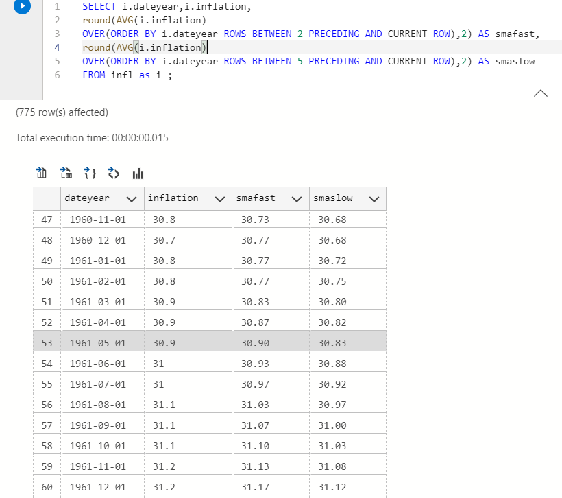
If the 3 month moving average is higher than the 6 month moving average than the CPI is moving faster as of late.
Calculating percent change in inflation each month
Most people are familiar with (y – x / x ) to calculate percent change, I use (y/x) -1 here. They give the same result because math. I multiply the result by 100 to make it a percentage.
SELECT i.dateyear,i.inflation,
lag(i.inflation)
OVER(ORDER BY i.dateyear) AS lagged,
round(((i.inflation / lag(i.inflation) OVER(ORDER BY i.dateyear))-1) * 100,4) as perchange
FROM infl as i ;
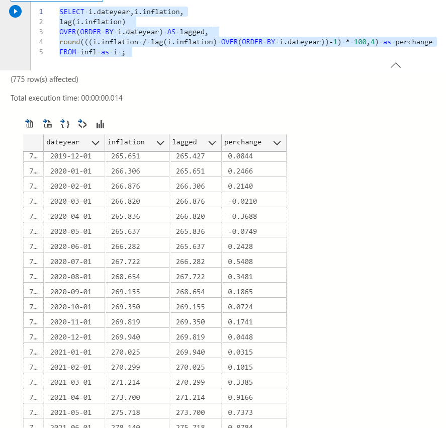
You will notice CPI has recently gone up larger precents.
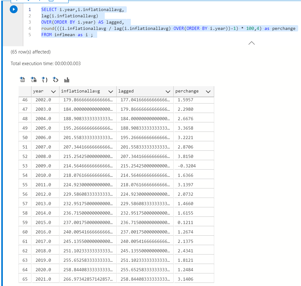
Looking at the annual values would be a bit more useful since monthly numbers probably vary a lot. PSQL has a variance function if you’re curious and want to try it yourself.
Earlier we saved a View for the average annual CPI numbers which allows finding the annual percentage change easily.
SELECT i.year,i.inflationallavg,
lag(i.inflationallavg)
OVER(ORDER BY i.year) AS lagged,
round(((i.inflationallavg / lag(i.inflationallavg) OVER(ORDER BY i.year))-1) * 100,4) as perchange
FROM inflmean as i ;
Other useful statistical summary functions
I suppose mode() and median() can be tricky to calculate. They are called ordered set aggregate functions. They require a WITHIN GROUP statement ORDERED BY some column.
Median is the 50th percentile and mode is the most frequently occurring value.
SELECT EXTRACT(year FROM dateyear) AS year,
min(i.inflation),
avg(i.inflation),
max(i.inflation),
count(i.inflation),
sum(i.inflation),
mode() WITHIN GROUP (ORDER BY i.inflation),
percentile_cont(.5) WITHIN GROUP (ORDER BY i.inflation) as median
FROM infl as i
GROUP BY year
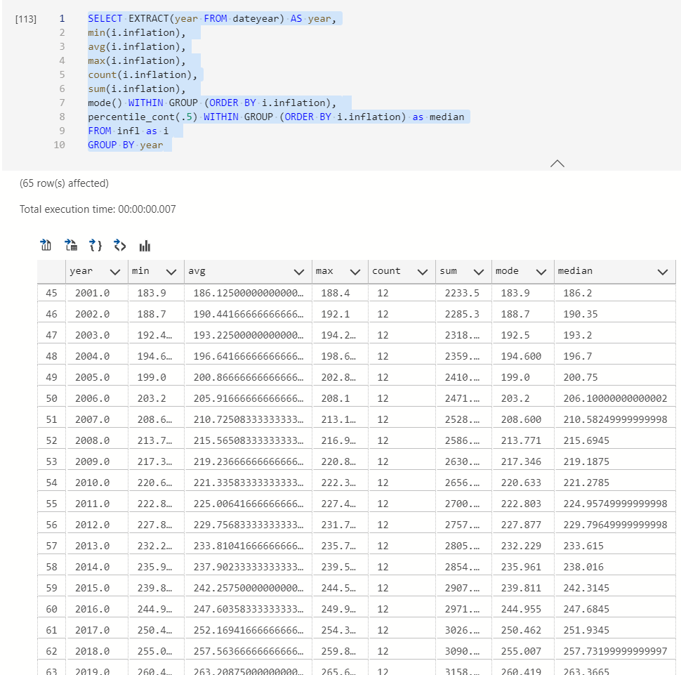
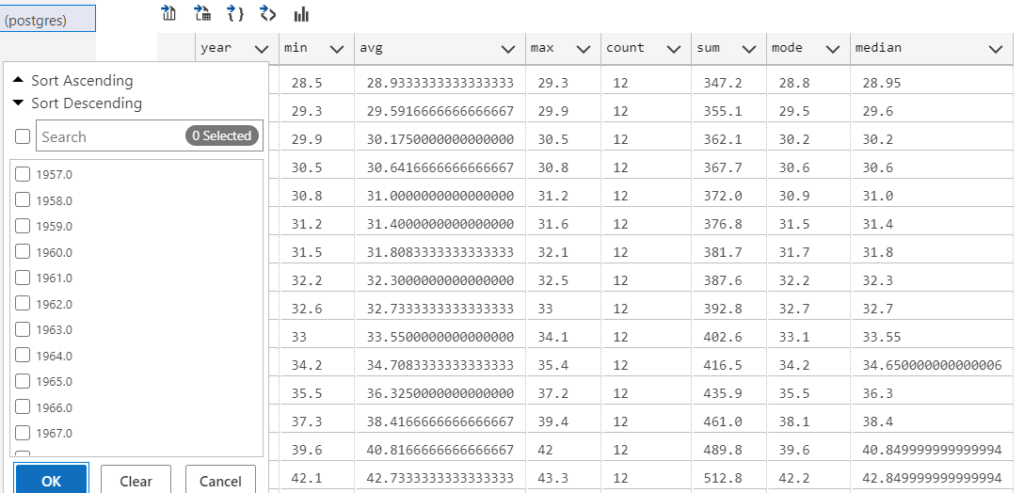
The results have a filter button. You can always slice the values between a period if your dataset is too huge or if you’re too lazy to write it into your query.
Sometimes for EDA it’s nice to get all the data and look at different periods via GUI. However, I mostly use SQL to fetch data and Python for EDA.
Ranking where we are in terms of historical CPI
If we rank by CPI it wont provide an accurate answer because CPI increases every year. Central banks even have an annual inflation target, so it’ll be very boring to look at.
A smarter way would be to rank the percentage change each year.
select i.year,i.inflationallavg,i.perchange, rank() over(ORDER BY i.perchange DESC) as rank
FROM inflrank as i
WHERE i.perchange is not null
ORDER BY rank ASC
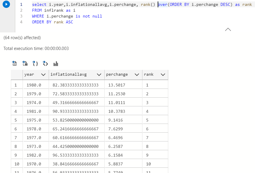
COOL! unsurprisingly the highest percentage change was during the 1980s, it was inflationary af. Many of you probably don’t remember the economic recession then, I don’t either but I’m a student of economics. Sharp rise in energy prices and tightening monetary policies caused severe inflation and made the economic recession worse.
Quick Google search says our number is also pretty accurate, I would hope so since it came from the FED.
AMAZING WORK!
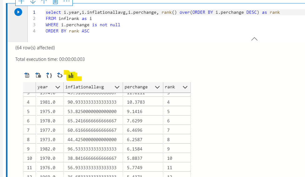
Bonus: Poor visualisation in Data Studio
Unless you’re used to seeing a lot of tables you probably need some charts. If you’re a product manager then you definitely need them for your stakeholders.
You can click this magic button to make simple charts.
It’s horrible and you need to structure your query exactly how you want the chart to work. The first column can be used as a row label in settings.
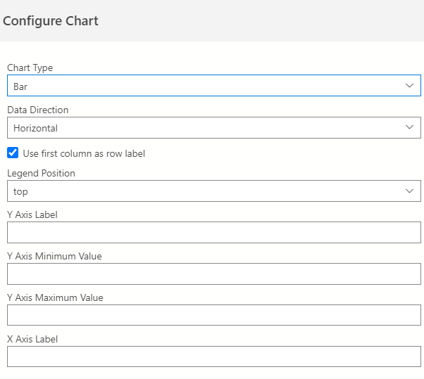
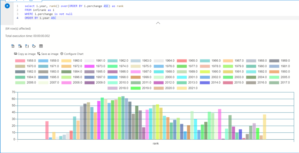
I don’t recommend. But if you need a simple bar chart with a ridiculous legend to annoy someone then you can use this.
What you learned
- Modern tools for SQL querying that let you save your queries in a convenient notebook.
- Making a table, adding values and dropping a table.
- Importing .CSV files
- Joins
- Views and some advanced queries using lag and ordered sequence functions
- Finding patterns, it helps to visualise the data
What you can learn
- All the different data types and in built functions
- Using software on top of Postgres like Timescale DB
- Connecting and running the server on a cloud platform
- Go through the documentation and click whatever you find of interest.
References