Hey.
Many people are familiar with MNIST, if you aren’t then it is a dataset consisting of handwritten digits from 0 to 9. It stands for Modified National Institute of Standards and Technology.
It’s frequently used in training computer vision models to benchmark various classification algorithms. Grad projects and research papers alike use it to show the accuracy of various models. There are research papers on arXiv, a popular repository for new computer science papers that use MNIST, even in August 2021.
I often see people use MNIST to ‘test out’ models. However, it doesn’t mean much and people reading papers that use MNIST from the past decade should critically think about the content or try testing it on another dataset.
Why fashion MNIST?
If you’re starting out with computer vision and want to try out different archetecture then you can already get in the good habit of moving away from MNIST.
Fashion MNIST is a more complex dataset that contains apparel labelled for your convenience.
Maybe you wear fedoras (not ironically) and would like to improve extend your sense of fashion. Maybe you’re into high fashion, or even urban fashion and would like to work with a cool dataset.
Check out this high top!
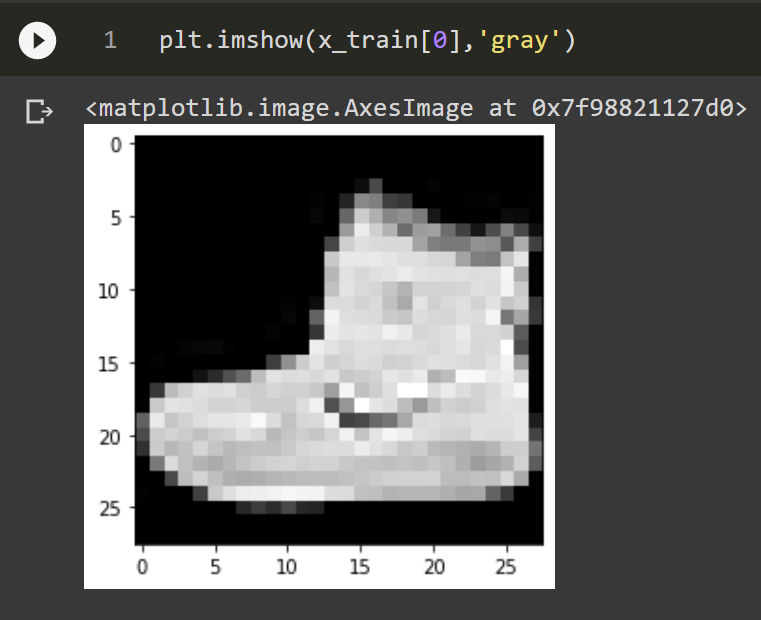
If the shoe didn’t impress you then here are a few reasons why handwriting recognition on digits is not enough to compare computer vision models nowadays.
- MNIST is too easy, many models can be 99% accurate in recognising digits.
- Most digits can be distinguished by a few pixels.
- It’s not representative of most things start-ups are trying to achieve.
- Many good ideas work on MNIST, so do many bad ideas.
- Also, many good ideas like batch normalisation don’t work well on MNIST or so I hear.
- Recognising apparel is cooler then recognising handwritten digits.
How to get started with using fashion MNIST?
Each pixel can be represented as a different intensity value from 0 to 255. Values closer to 0 mean darker and vice versa. I had written a brief introduction to images and how you can figure out their intensity by looking at the histogram of pixel values in the following article.
We can load these images and use their matrix representation to train a model. The data comes by default with TensorFlow. The images can also be downloaded them from the GitHub repository of Zalando Research, a German e-commerce company that created the dataset. I’ll link the GitHub at the bottom but I recommend using it from TensorFlow or other machine learning libraries that have it.
Google Colab to use avoid installing TensorFlow locally
To mix it up I used https://colab.research.google.com/ which will allow running notebooks in the browser. It should be easier for beginners that don’t have a local environment. All you need is a Google account, your notebook can be shared or exported to use locally later.
If you want to use Python locally follow this article: https://freshprinceofstandarderror.com/ai/setting-up-your-data-science-environment/
Anyway, type this in Collab to import TensorFlow, numpy and your favourite plotting library.
import tensorflow as tf #DL library by google
import numpy as np #computation with arrays
import matplotlib.pyplot as plt #creating visualisations
TensorFlow comes with Keras since version 2, we can use it to load fashion MNIST.
(x_train_full, y_train_full) , (x_test, y_test) = tf.keras.datasets.fashion_mnist.load_data() #imports the fashion mnist dataset
These are the labels in text, because y_ data has them in numbers.
class_names = ['top','trouser','pullover','dress','coat','sandal','shirt','sneaker','bag','ankle boot']
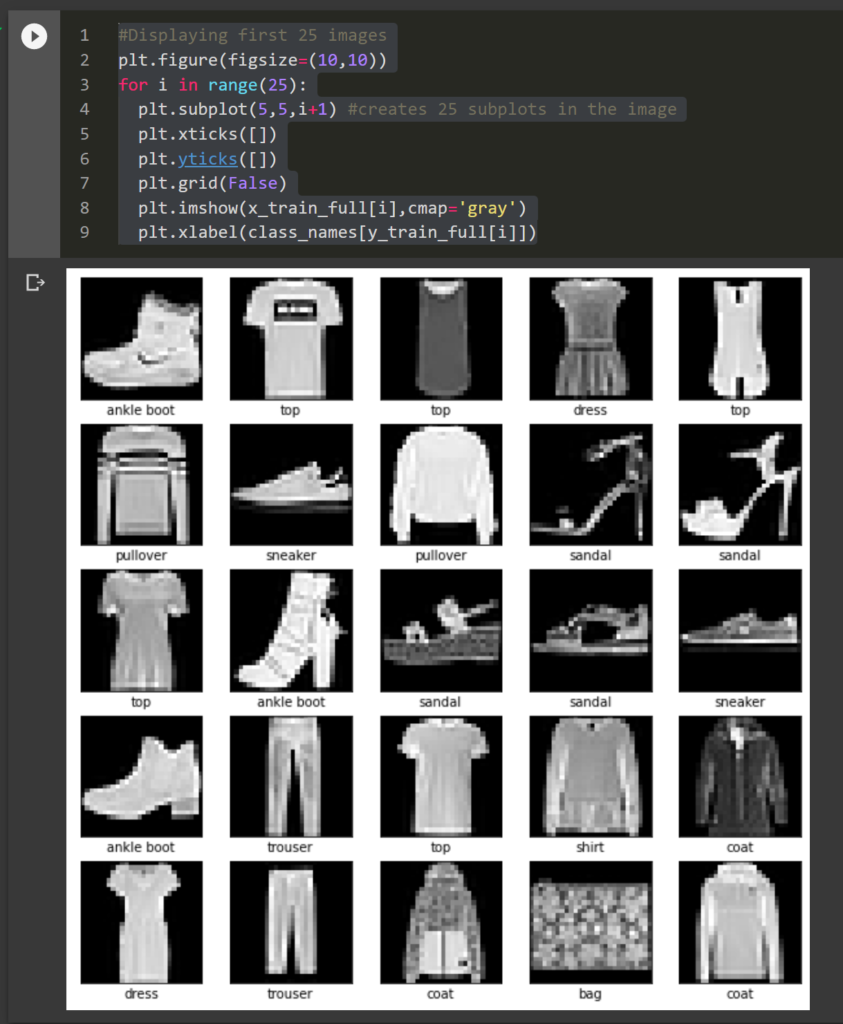
See the first 25 images for fun.
#Displaying first 25 images
plt.figure(figsize=(10,10))
for i in range(25):
  plt.subplot(5,5,i+1) #creates 25 subplots in the image
  plt.xticks([])
  plt.yticks([])
  plt.grid(False)
  plt.imshow(x_train_full[i],cmap='gray')
  plt.xlabel(class_names[y_train_full[i]])
Nice work, I feel bad leaving it at just this though.
Simple neural network in Keras
If you’ve come this far might as well go a step further by making a small neural network. There are a lot of good courses on neural networks so I’ll keep it brief because I don’t want to publish the same stuff as everyone else.
We’ll make it simple but interesting, maybe 3 layers with the last being a Softmax layer. A Softmax layer provides probabilities for all the classes. These probabilities add up to 1. The class with the highest probability is considered the right(est) class. If the model believes a garment could be both a sock and a shoe then it would give both of them a probability of .5 and everything else a probability of 0. If you don’t understand it then you’ll get to see the numbers soon enough.
To give this model a fighting chance we’ll normalise the numbers from 0 to 1 by diving everything by 255.
#Normalising data between 0 to 1
x_valid,x_train = x_train_full[:5000] / 255.0 , x_train_full[5000:] / 255.0

y_valid, y_train = y_train_full[:5000],y_train_full[5000:] #y does not need to be normalised; labels for apparel

x_test = x_test / 255.0
We’ll define the layers, loss function and optimiser next.
model = tf.keras.models.Sequential([tf.keras.layers.Flatten(input_shape=[28,28]),
                                    tf.keras.layers.Dense(300,activation='relu'),
                                    tf.keras.layers.Dense(100,activation='relu'),
                                    tf.keras.layers.Dense(10,activation='softmax')
                                    ])
model.compile(loss='sparse_categorical_crossentropy',
optimizer='sgd',
metrics=['accuracy'])Fit the compiled model on the train sets and provide it with the validation data.
history = model.fit(x_train,y_train,epochs=50,validation_data=(x_valid,y_valid))
This is how we can see the accuracy.
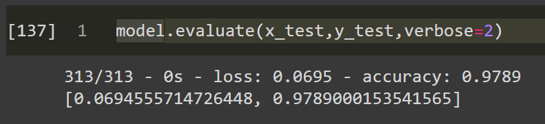
model.evaluate(x_test,y_test,verbose=2)
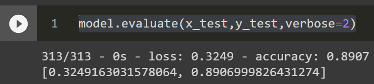
It’s close to 90% accurate, I guess it wasn’t too bad. Unlike regression and other machine learning, classifying images can get a high accuracy score, because most shoes are similar to each other etc.
This is how we can classify an image with the model we trained.
probability_model = tf.keras.Sequential([model,
                                         tf.keras.layers.Softmax()
                                         ])

predictions = probability_model.predict(x_test)
Interpreting the predictions can be challenging if you don’t understand SoftMax.
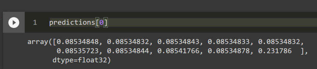
These probabilities add up to 1, there are 10 of them because we have 10 classes. The highest probability in this case is .231 which relates to the 10th class, which was ankle boot.
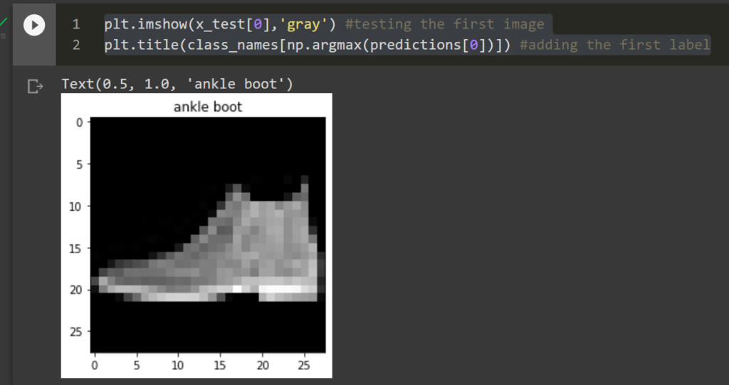
Lets see the image that was classified as ankle boot.
plt.imshow(x_test[0],'gray') #testing the first image
plt.title(class_names[np.argmax(predictions[0])]) #adding the first label
Using the same model on MNIST would probably get us a near perfect accuracy. Change the dataset from fashion MNIST to MNIST and try it for yourself.
You can change the dataset easily like so.
(x_train_full, y_train_full) , (x_test, y_test) = tf.keras.datasets.mnist.load_data()
Almost 98% accurate! Even a hedge fund quant can look like a computer vision expert from Deep Mind or Tesla when using MNIST.
What you learned?
- Simple is good, but some datasets have become too simple even for models you can make up in 5 minutes.
- It’s better to try to solve problems that organisations are facing, Fashion MNIST is still simple but with enough complexity like tasks at an actual workplace.
- I don’t like MNIST