
Merry!
I bring presents regardless of whether you celebrate the birth of Isaac Newton… according to the Julian calendar.
I know everyone is excited to peruse math over the holiday period.
Anyway, on the first day of Christmath your good friend brought to you a song and a math.
December 25th: Day 1
Area of a Circle ft. Change of Variables
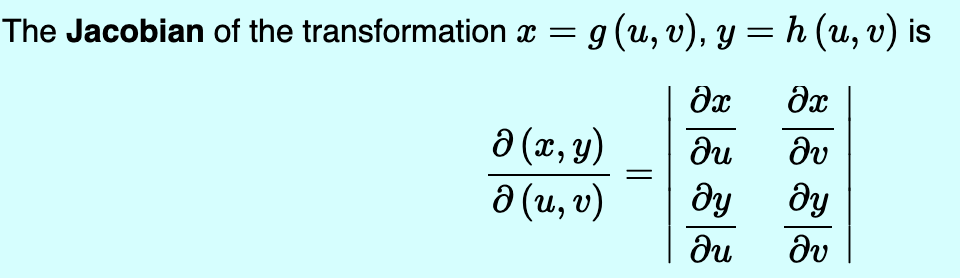
Maybe this is a tougher one but it’s also the most satisfying. It requires some knowledge of the Jacobian, double integration and polar coordinates. I know all the cool kids might pretend this is high school math but I’ll save you the deception. If you find this one too hard, I promise the others will be simpler.
If you took undergrad linear algebra then you might be familiar with matrices. The Jacobian is a matrix of first order partial derivatives. I never took vector calculus, I actually learned it in mathematical statistics. Its determinant is used to transform functions like the probability density function via the change of variable formula.
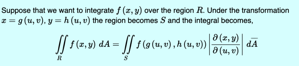
ANYWAY to find the area of a circle we need π r2 to double integrate dx dy. Which seems like a pain in cartesian coordinates but not in polar coordinates. Thus the use of change of variables formula.
Now that we have all the required info let’s begin.
\int \:\int \:dxdy
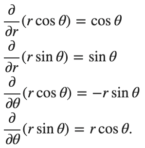
let x\:=\:r\:cos\:\theta \:and\:y\:=\:r\:sin\:\theta
We need the dxdy (infinitesimal bit) in terms of r and θ. Therefore we use the change of variables formula for which we need the determinant of the Jacobian. I used symbolab for the partial derivatives because I’m lazy smart. You can find the derivatives one by one and get the following Jacobian.
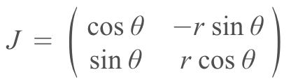
We need its determinant, which is conveniently r.
Now we just evaluate with the limits, and magic.
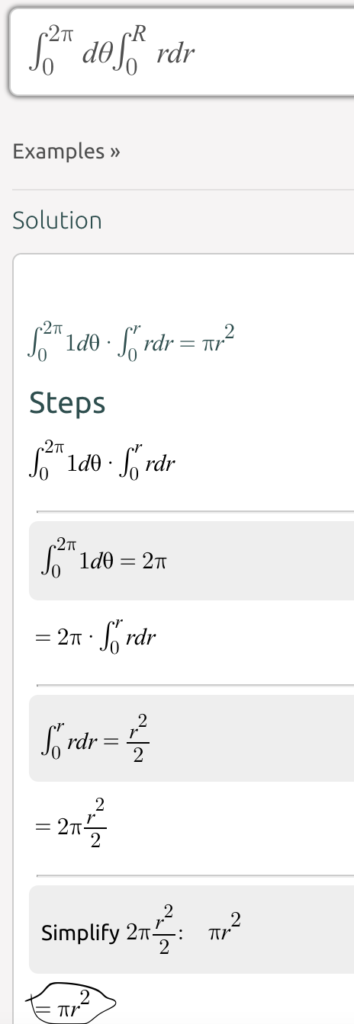
= \int _0^{2\pi }\int _0^R\:rdrd\theta we can factor this
= \int _0^{2\pi }d\theta \:\int _0^R\:rdr
= \pi \:r^2
If the last part was too quick for you have a look at this.
References:
These don’t have the area of a circle but the second one is closeish.
- https://tutorial.math.lamar.edu/classes/calciii/changeofvariables.aspx
- https://mathinsight.org/double_integral_change_variable_examples
December 26th: Day 2
Little’s Law or Little’s Result, Little’s Lemma, Little’s Formula.
This ‘law’ is a favorite because of its simplicity. It is popular in queuing theory and I learned it in operations management during my MBA. The first proof by John Little was considered a complicated stochastic proof but the law/result/lemma is as follows:
L = λ * W
L = Work-in-progress (WIP) which is the average number of items in a queuing system
λ = Throughput which is the average number of items arriving or departing per unit of time
W = Lead time which is the average waiting time an item spends in a queuing system
I remember it by “inventory = flow rate * flow time” and it can be rearranged to suit your needs. It’s a relatively modern discovery and has fairly accurate results in stationary data. It can be applied to individual queues and also networks and subnetworks.
For example: How long will it take you to respond to emails if on average you write 60 emails a day and have to respond to 240 emails?
240 = 60 * W
W = 4
Let’s go for a more complicated one.
In a large Melbourne hospital 10 COVID patients are admitted to the ICU each day. 80% of the cases stay in ICU for 2 days and 20% stay for 5 days.
What is the average occupancy for the ICU ward?
We know know the flow is 10/day. The flow time is a weighted average. With two pieces of information we can calculate the third.
λ = 10 per day
W = .8 * 2 + .2 * 5
L = λ * W
L = 10 * 2.6
L = 26
The ICU ward usually has 26 COVID patients. Or an average occupancy of 26.
It feels pretty intuitive, obvious and simple. But it is not often applied unless trained in the sciences of operations management. You would also be ill-advised to build an ICU with only 26 beds, this is an average and some days would be higher. The distribution for COVID cases would also not be stationary. Like any power, use your math responsibly.
Reference :
https://people.cs.umass.edu/~emery/classes/cmpsci691st/readings/OS/Littles-Law-50-Years-Later.pdf
I want to write about these sometime in the future.
Random Matrix Theory ft. Marchenko-Pastur Theorem
Eigenvalues Using Trace and Determinant
Approximation for Exponential Moving Averages
One-Shot Linear Regression
Elasticity
Bayesian Regression vs Ridge and Lasso Regression
Norms and Error
Central Limit Theorem Using Resampling Methods
Inner Products ft. Dot Product
Portfolio Volatility