
Hey,
Do you need to retrain a large language model on your 2 year old potato laptop? Sorry, we still need a lot of computing power. While in many cases retraining or even running large models on your M1 MacBook Air is unachievable; we might be getting closer thanks to clever linear algebra.
LoRA and QLoRA are the cool kids in in parameter-efficient fine-tuning (PEFT). Q stands for quantization, instead of representing parameters in 32 bits you can represent them with less precision in fewer bits making it even more efficient than LoRA.
In the LoRA (Low-Rank Adaptation) paper the authors compared fine-tuning with the traditional method of retraining the entire model vs LoRA. In one case they reduced the VRAM consumption during training from 1.2TB to 350GB, sped up training and didn’t add additional latency during inference. I’ll link the original paper that was authored by the fine people at Microsoft at the end.
Don’t worry if this makes no sense yet.
The main idea.
Imagine you have a big LEGO castle. It’s huge, and it took you a long time to build. Now, let’s say you want to make a small change to the castle. You could undo all your work and start building again, but that would take so much time, right? Instead, what if you had a mini LEGO set that you could simply add to your castle, without having to start over? That’s where decomposed matrices come in. These are like our mini LEGO sets. Instead of changing the model’s parameters that might be billions of little bricks, we can add these adapters (low rank matrices) to influence the model’s behavior.
Fine-tuning lower rank matrices, which can be added to the original weight matrix lets us teach the model new things or amplify things it may already know from pre-training. Why is it better to have low rank decomposed matrices? B and A have fewer values in them than W so training takes less time because you need to compute fewer gradients. In the past parameter efficient fine tuning really meant freezing the original layers and adding a couple of new layers which added latency. LoRA has zero added latency during inference since you can fuse the LoRA weights into the model thus not increasing the size or having to do additional layers worth of computation.
Well libraries do all of this for you and more but that is how they work behind the scenes. There are a few minor details like ∆W = BA and the formula takes into account the input (W+ BA)x or Wx + BAx. The fine-tuned low rank matrices are called adapter modules. One of the ways to have a smaller BA is to decompose the weight matrix using SVD (singular value decomposition). You reduce the rank by keeping the most important singular values etc. If you understand the intuition by the end of this then reading the paper will be easier. Look at the last section where we will decompose a matrix and that will help the intuition stick.
Relevant anecdote
When I studied deep learning at university we were introduced to transfer learning early on; you can have a huge model that is a general learner like VGG16 or ResNet but fine-tune it to specific downstream tasks or ‘instruction tune’ it. In most cases you just freeze the original model parameters and train very few new ones by adding a new layer towards the end. This approach always felt intuitive. Parameter Efficient Fine-Tuning until recently meant freezing most parameters and training a few adapter layers at the end.
These ideas aren’t mutually exclusive, you can still only train fewer parameters (like only attention ones) and you can decompose whatever matrix into n matrices that have fewer total values. I think the really exciting part about LoRA is that instead of adding an adapter layer sequentially we have the adaptor in parallel thus avoiding latency in the final fine-tuned model.
Basics of Matrix Decomposition
Okay finally, if you never took linear algebra you might be asking: What are decomposed matrices? What is a rank and how can something become lower rank?
Remember when you were 5 years old and had 1000 crayons? Then you realised a lot of those crayons were close in colour and you could just use 3 crayons to recreate your masterpiece rainbow drawing. It’s the same thing.
While you probably can’t learn linear algebra from this article, these are simple explanations for words people might use.
Linear Combination: It’s just a mix, like combining crayons of different colors gives you a new shade of crayon depending on how much of each crayon you used. Formally it’s taking several vectors and combining them using scalar multiplication and vector addition. If you add 2 vectors like v_1 and v_2 it is a linear combination (the scalar is 1 so 1*v_1 + 1*v_2).
Rank: It tells you how many unique dimensions or directions exist in your matrix. If you can use the primary colored crayons to make all the other 997 crayons then you just have rank 3. The rank is all about linear independence and span. Those 3 linearly independent crayons/vectors can combine to create many other ones but they will only span the palette/space possible to reach with those 3 crayons/vectors.
Matrix decomposition: Sometimes a big puzzle can be broken down into two small ones. The two small puzzles might be easier to work with and you can always combine them to get the bigger puzzle.
SVD: A type of matrix decomposition called Single Value Decomposition. One of the most important ones. It breaks down a matrix into 3 separate matrices A=UΣV*. It’s used in signal processing, compression and all the fun things people do with math. Σ is a diagonal matrix that contains singular values. The larger the singular value the more important it is in describing the matrix. Maybe I should show this in Python.
Power of Linear Algebra
Alright, open your Python files.
We’ll just need numpy.
import numpy as np
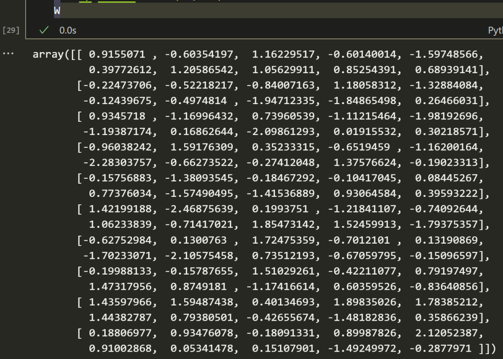
Let’s make a random matrix that is 10×10 or has 100 values. Pretend it’s the weight matrix or what people call the trainable parameters.
np.random.seed(69)
W = np.random.randn(10, 10)
W
Let us decompose the matrix using SVD.
U, S, VT = np.linalg.svd(W)
If we look at S we’ll see the singular values that are most important.
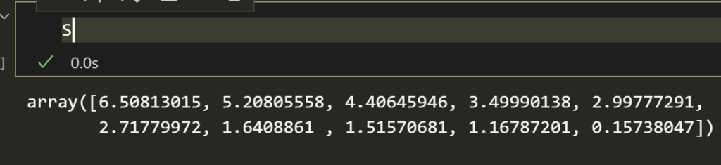
In this case the first 4 singular values are nice and large. Reduce the rank to 4 or whatever k you pick.
k = 4  # Rank of the approximation

# Only keep the top k singular values
S_k = np.diag(S[:k])

# Take only the first k columns of U and rows of VT
VT_k = VT[:k, :]
B = U[:, :k]
A = np.dot(S_k, VT_k)

# Low-rank approximation
BA = np.dot(B, A)
Cool, now you might notice B and A are less than 100 values. We can check their shapes.
print(f'W shape {W.shape}, B shape {B.shape}, A shape {A.shape}')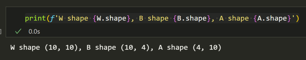
Awesome, so while the original matrix was 100 values (10*10 matrix), the new ones add up to only 80 values (10*4 and 4*10). In reality if the matrix you are decomposing is extremely dense with a lot of weights that don’t need to be there then you’ll see better efficiency. This is because you can pick a pretty low rank since many of the values don’t need to be in there to approximate the matrix. In a large language model or most deep learning models this is the case since a lot of noise is also captured within the weights.
We can compare how close it is to our original matrix.
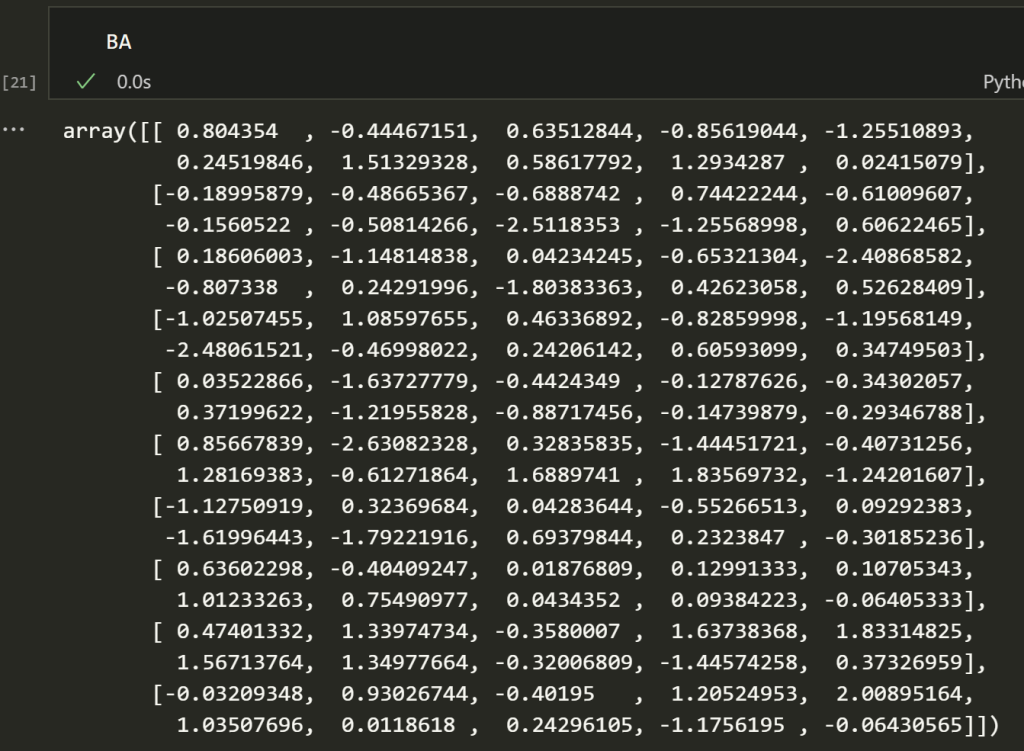
It’s closeish, but we eyeballed the rank and this is going to be trained on a new task anyway. You could always take the Frobenious norm of the difference between the two and check the quality of the approximation.
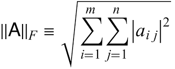
# Check the quality of the approximation
error = np.linalg.norm(W - BA, 'fro')
print("\nFrobenius norm of the difference:", error)
Yeah it looks okay. We’re not actually going to use the approximate matrix as a replacement for the weights. We’re going to be training it.
We can do a quick review on quantization or the main idea behind QLoRA.
By default our matrix is float64 which is 8 bytes per value.
W.dtype.itemsize
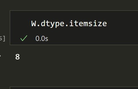
If we multiply that by number of elements we get the size of the matrix. We can divide it by 1024 to get the size in KB.
def numpy_array_size_in_kb(array):
    element_size = array.dtype.itemsize
    num_elements = array.size
    size_in_bytes = element_size * num_elements
    size_in_kb = size_in_bytes / 1024
    return size_in_kb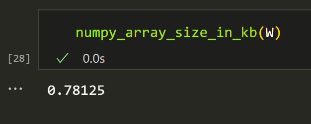
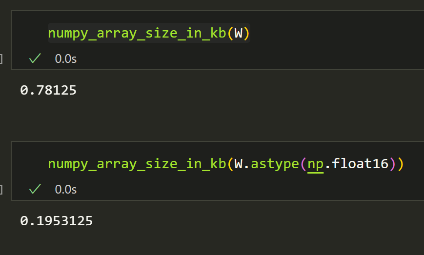
So the main idea behind QLoRA or quantization is that we can convert it to a smaller type and have a smaller matrix size. What a shock. For example float16 would be 2 bytes instead of 8.
W.astype(np.float16).itemsize
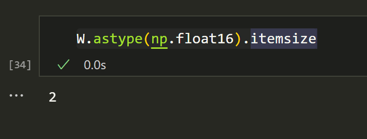
We can put it in the same function as earlier.
numpy_array_size_in_kb(W.astype(np.float16))
That is as expected, as massive reduction in size.
Awesome, nice work. So we learned, lower rank decomposed matrices can have fewer values than the original weight matrix. Casting numbers to types that need less memory also takes less space.
Congratulations; you now understand the intuition behind LoRa and QLoRA.
Things to learn next
- Using the PEFT and Transformers library from hugging face
- Thats probably it.
- Maybe read this paper https://arxiv.org/abs/2106.09685